Programming Model
I. Programming Model Overview
1.1 History
- 2001/2002, researchers see GPU as data parallel coprocessor, the GPGPU field is born
- 2007, NVIDIA releases CUDA
- CUDA – Compute Unified Device Architecture
- 统一计算设备架构
- GPU shifts to GPGPU for computing
- Graphics 编程 → General-Purpose 编程
- 2008, Khronos releases OpenCL specification
1.2 GPGPU Programming Model
一个编程模型应该包含:
- How to compute the wanted function
- 如何组织 memory 为计算服务
- How to map the function to the real hardware
此外,对于并行架构,尤其重要的是:
- How to divide the workload(如何划分工作量)
- How to communicate between the divided work(如何在划分的工作之间进行通信)
- How to synchronize the divided work(如何同步划分的工作)
也就是说,GPGPU programming model 要能说明:在每一个时刻,每个 SM 中的每个 CUDA Core 应该做什么。
II. NVIDIA Programming Model: CUDA
2.1 Computing Model
CUDA 使用的是异构计算(heterogeneous computing)模型:程序员写出的 GPGPU 应用程序会被分成两类代码:
- Host code:运行在 CPU 上的主机端代码
- Device code:运行在 GPGPU 上的设备端代码
从程序员视角看,一次典型 CUDA 执行流程如下:
- CPU 先把 processing data 从 main memory 拷贝到 GPU memory
- CPU 发出指令,告诉 GPU 要执行什么并行计算
- GPU 在多个 core 上并行执行
- 计算结果再从 GPU memory 拷回 main memory
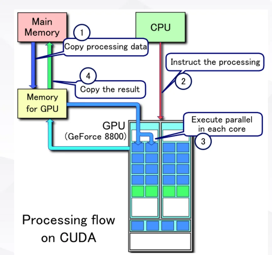
CPU 通过 kernel 来调用 GPU。kernel 在 CUDA 的线程层级中也可以理解为一个 thread grid:
-
CPU: __host__:指定代码在 CPU 上做 -
CUDA: __global__:定义从 host 启动、在 device 上执行的 kernel -
CUDA: __device__:定义在 device 端调用、在 GPU 上执行的函数
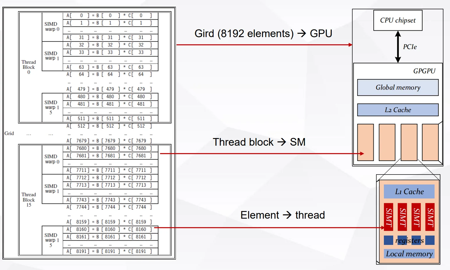
注意,逻辑执行与 GPU 硬件的映射关系是:
-
kernel (grid)(线程网格) \(\rightarrow\) GPU -
thread block(线程块) \(\rightarrow\) SM -
thread(线程) \(\rightarrow\) SP / CUDA Core(逻辑对应,实际执行以warp(线程束) 为调度单位)
kernel launch 的基本写法是:
其中:
-
dimGrid:一个 grid 里有多少个 thread block -
dimBlock:一个 thread block 里分配多少个 thread
例如向量逐元素相乘:
这里的含义是:把 8192 个元素划分成 16 个 thread block,每个 thread block 有 512 个 thread。也可以换成其他满足总线程数需求的配置(例如 8 x 1024),但实际可行的 dimBlock 会受硬件最大线程数、寄存器、shared memory 等资源限制。
2.2 Thread Model
2.2.1 Thread Hierarchy
CUDA 的线程层级是:
- Grid:线程网格
- Thread block:线程块
- Thread:线程
对应到程序里的内置变量:
-
gridDim(x, y, z):一个 grid 中 block 的维度,也就是“一个 grid 有几个 block, \(x,y,z\)的 范围是多少” -
blockDim(x, y, z):一个 block 中 thread 的维度,也就是“一个 block 有几个 thread, \(x,y,z\)的 范围是多少” -
blockIdx(x, y, z):当前 thread 所在 block 的编号,也就是“当前 thread 在 grid 中的 block 编号” -
threadIdx(x, y, z):当前 thread 在 block 内部的本地编号
2.2.2 Example
Example 1: 数组元素按照线程分配
如果只看一维数组(即假设所有层次均是一维网格),最常用的全局下标计算方式是:
这句话可以拆成:
-
blockIdx.x * blockDim.x:前面已经经过了多少个完整 block -
threadIdx.x:当前 thread 在本 block 内的本地编号 - 两者相加得到当前 thread 对应的一维全局下标
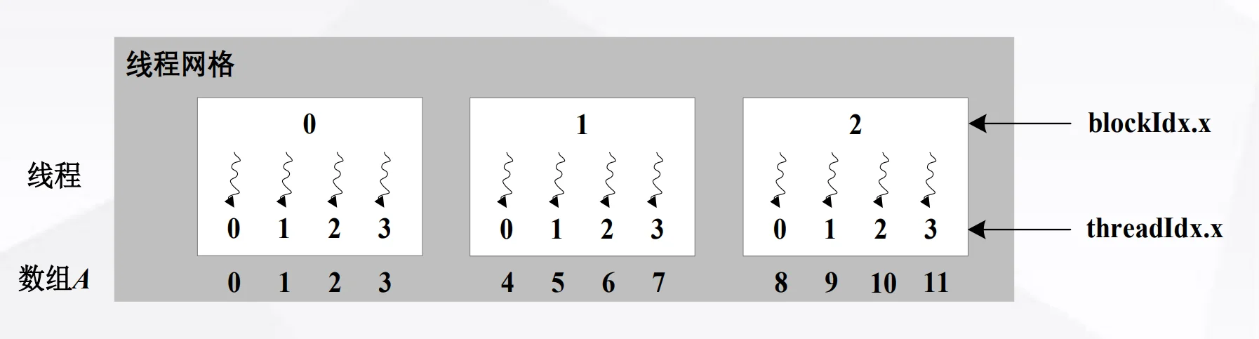
__global__ void kernel1(int* A) {
    int index = threadIdx.x + blockIdx.x * blockDim.x;
    A[index] = index;
}
// kernel1 结果:0 1 2 3 4 5 6 7 8 9 10 11

__global__ void kernel2(int* A) {
    int index = threadIdx.x + blockIdx.x * blockDim.x;
    A[index] = blockIdx.x;
}
// kernel2 结果:0 0 0 0 1 1 1 1 2 2 2 2

__global__ void kernel3(int* A) {
    int index = threadIdx.x + blockIdx.x * blockDim.x;
    A[index] = threadIdx.x;
}
// kernel3 结果:0 1 2 3 0 1 2 3 0 1 2 3
复习时可以这样记:
-
index是全局连续编号 -
blockIdx.x在同一个 block 内相同 -
threadIdx.x在每个 block 内从 0 重新开始
Example 2: Vector Multiplication
向量逐元素相乘的例子是:
__global__ void vect_mult(int n, double *a, double *b, double *c)
{
    int i = blockIdx.x * blockDim.x + threadIdx.x;
    if (i < n) {
        a[i] = b[i] * c[i];
    }
}
host code 调用:
这个配置的含义是:
- Grid:8192 elements -> 8192 threads
- 16 thread blocks
- 每个 thread block 有
8192 / 16 = 512threads
注意 if (i < n) 的含义:如果元素数不是线程数的整数倍,例如只有 8191 个元素,但是我们依旧会按照 \(16\times 512=8192\) 分配,最后多出来的 thread 会因为这句判断而不访问数组,从而防止越界。
当硬件资源不够时会发生什么?
例如每一个 SM 只有 32个 SP?
——需要时分复用!
\(512/32 = 16\) warps,因此会构建 16 个 warp(线程束)。每一个时刻独立执行 1 个 warp,其他 warp 处于等待状态,等当前 warp 执行完毕后再切换到下一个 warp。
Thread mapping to hardware
Example 3: Matrix-Vector Addition
课件的第二个 CUDA 例子是矩阵加向量广播:
指定划分方式:
- 每个 Thread Block 负责一个 \(H\times W = 128\times 32\) 的 tile
- 每个 tile 由
threadsPerBlock(16, 8)个 thread 处理 - 因此:每个 thread 计算 \((32/16) \times (128/8) = 2 \times 16\) 个元素
device code 的关键下标计算是:
int row_start = blockIdx.y * blockDim.y * 16 + threadIdx.y * 16;
int col_start = blockIdx.x * blockDim.x * 2 + threadIdx.x * 2;
(1) 拆解:每一个 thread 处理 16 行数据,
blockDim.y是一个 thread block 的 thread 的行数,blockIdx.y是当前 block 在 grid 中的行编号。blockIdx.y * blockDim.y * 16就表示当前 thread block 的起始行号,threadIdx.y * 16表示当前 thread 在 block 内的行偏移。
(2) 列的计算同理。
然后每个 thread 用两层循环完成自己的 [2, 16] 小块:
for (int i = 0; i < 16; ++i) {      // 16 rows
    int row = row_start + i;
    if (row < numRows) {
        for (int j = 0; j < 2; ++j) {   // 2 columns
            int col = col_start + j;
            if (col < numCols) {
                matrix[row * numCols + col] += bias[col];
            }
        }
    }
}
这里的 if (row < numRows) 和 if (col < numCols) 是为了处理边界情况:当矩阵的行数或列数不是 128 或 32 的整数倍时,最后一个 tile 会有一些线程对应的行或列超出矩阵范围,这些线程就不进行计算。
host code 中的配置是:
dim3 threadsPerBlock(16, 8);
dim3 blocksPerGrid((numCols + 31) / 32,
                   (numRows + 127) / 128);

matrixAddBiasLargeTile<<<blocksPerGrid, threadsPerBlock>>>(
    d_matrix, d_bias, numRows, numCols
);
这里 (numCols + 31) / 32 和 (numRows + 127) / 128 是向上取整。例如:如果 numCols = 63,应该划分为两列线程块,普通整数除法 63 / 32 = 1 会少算一块,但 (63 + 31) / 32 = 2,正好覆盖剩余列。
2.3 Memory Model
2.3.1 GPGPU 中的 Memory Hierarchy
Memory model 的基本思想是:根据数据的访问需求选择合适的存储层次,尽量减少对 global memory 的访问。
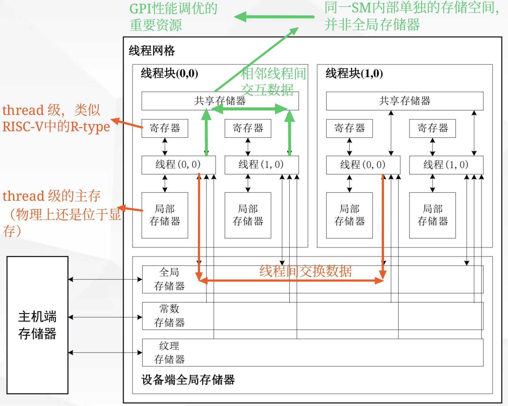
当前 CUDA memory model 中常见的类型包括:
- Register file:寄存器文件,每个 thread 私有,速度最快,用来放线程内部的临时变量
- Local memory:局部存储器,每个 thread 私有;名字叫 local,但物理上通常仍在设备端全局存储器中,只是逻辑上属于某个 thread
- Shared memory:共享存储器,同一 thread block 内线程共享,位于同一 SM 内部的单独存储空间,并非全局存储器
- L1 data cache:类似之前 RISC-V 处理器中学过的 Cache,由硬件管理
- Global memory:设备端全局存储器,所有 thread 都能访问,但访问代价高
- Constant memory:常量存储器,物理上也在设备端全局存储器中,适合只读常量数据
- Texture memory:纹理存储器,物理上也在设备端全局存储器中,有专门的缓存/访问路径
注意关注Shared memory:
- 是 GPGPU 性能调优的重要资源
- 它由程序员显式控制,而不是像 cache 一样完全交给硬件
- 它可以服务于同一个 block 内线程之间的数据复用和通信
- 某些架构中,L1 cache 和 shared memory 会共享片上空间,可以动态调整划分;如果程序员愿意主动优化,就可以把更多片上资源作为 shared memory 使用,从而写出更高性能的 CUDA 程序
2.3.2 TLP 和资源限制
TLP(Thread-Level Parallelism)可以理解为:一个 SM 上能同时驻留、随时可被调度的 thread / warp / thread block 有多少。TLP 越高,SM 越容易在某些 warp 等待 memory 或长延迟指令时,切换去执行别的 warp,从而隐藏延迟。
注意:“驻留” 的含义是一个 thread block / thread 的运行上下文已经被分配到某个 SM 上,占用了这个 SM 的寄存器、shared memory、warp slot 等资源,等待或正在被调度执行。
关键点是:驻留并不等于正在执行。
但是,TLP 不是只由 kernel launch 时写了多少 thread 决定。一个 SM 能同时容纳多少工作,还会被以下因素限制:
-
# threads:一个 SM 最多能驻留多少 thread -
# thread blocks:一个 SM 最多能驻留多少 thread block -
Size of register file:每个 thread 使用越多 register,可同时驻留的 thread 越少 -
Size of shared memory:每个 block 使用越多 shared memory,可同时驻留的 block 越少
Example 1: V100 的资源限制
以课件中的 V100 / Volta GV100 为例:
- 每个 SM 最多
2048 threads - 每个 SM 最多
32 thread blocks - 每个 SM 有
256KB register file - 每个 SM 有最多
96KB shared memory
注意:课件里写的 256KB RF 是寄存器文件容量。因为一个 register 通常是 32-bit,也就是 4B,所以:
如果希望 SM 同时驻留满 2048 threads,平均每个 thread 能分到的 register 数量就是:
所以课件标注中的结论是:
- More regs needed, then less threads
- 如果一个 thread 需要超过 32 个 register,那么 V100 上这个 SM 就很难同时驻留满 2048 个 thread
shared memory 的思路类似。如果一个 SM 最多驻留 32 blocks,并且 shared memory 总量是 96KB,那么平均每个 block 只能用:
所以另一个结论是:
- More shm needed, then less blocks
- 如果一个 block 需要超过 3KB shared memory,那么一个 SM 上就不能同时驻留满 32 个 block
Example 2
课件中的具体 kernel 例子:
分别看三个主要限制:
(1) Register file 限制
每个 SM 的 RF 数量固定,每个 thread 分配的 RF 数 VS 可驻留的 thread 数
也就是说,如果每个 thread 要用 64 个 register,那么 register file 最多支持 1024 个 thread 同时驻留;每个 TB 有 128 个 thread,因此最多驻留 8 个 TB。
(2) Shared memory 限制
每个 SM 的 shared memory 总量固定,每个 block 分配的 shared memory VS 可驻留的 thread block 数
如果每个 TB 需要 8KB shared memory,那么 shared memory 最多支持 12 个 TB 同时驻留。
(3) 最大线程数限制
SM 限定的最大 TB 数 VS SM 限定的最大 thread 数以及每个 TB 的 thread 数
如果只看最大线程数,每个 SM 最多可以驻留 16 个这样的 TB。
最终一个 SM 上能驻留多少个 TB,要取所有限制中的最小值:
因此这个 kernel 在 V100 上的驻留 TB 数量由 register file 卡住,而不是由 shared memory 或最大线程数卡住。这个例子说明:写 CUDA kernel 时,
- 每个 thread 用太多 register 会降低可驻留 thread 数;
- 每个 block 用太多 shared memory 会降低可驻留 block 数;
- 两者都会降低 TLP。
2.4 Synchronization
并行程序需要同步,是因为多个 thread 之间经常存在数据依赖:一个 thread 先写入 shared memory,另一个 thread 后续要读取这个结果。如果没有同步,后读的 thread 可能在数据还没写完时就开始读取,得到旧值或未定义值。
2.4.1 Thread block 内同步
CUDA 中最基础的同步方式是 block scope 内的同步:
__syncthreads() 的含义是:同一个 thread block 内的所有 thread 都必须到达这个同步点,之后这些 thread 才能继续向下执行。下图里画的同步栅栏(barrier)就是这个意思:先到的 warp / thread 会在 barrier 前等待,直到 block 内其他 thread 也到达。
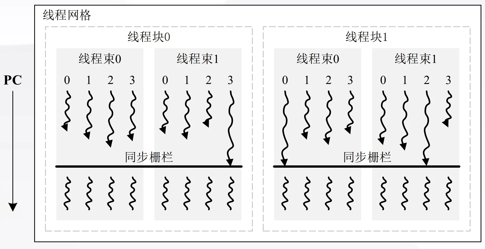
需要注意它的作用域:
-
__syncthreads()只能同步同一个 thread block 内部的 thread - 它不能同步不同 thread block,因为不同 block 可能被调度到不同 SM 上,甚至不一定同时驻留
- 对应到底层实现,可以理解为 CUDA 编译到类似
bar的同步栅栏指令
下面的矩阵乘法片段展示了为什么 shared memory 常常需要和同步一起使用:
__shared__ float Mds[BLOCK_SIZE][BLOCK_SIZE];
__shared__ float Nds[BLOCK_SIZE][BLOCK_SIZE];

Mds[tx][ty] = d_A[row * N + ty + i * BLOCK_SIZE];
Nds[tx][ty] = d_B[col + (tx + i * BLOCK_SIZE) * K];
__syncthreads();
这里每个 thread 负责把一部分 A 和 B 从 global memory 搬到 shared memory。只有当 block 内所有 thread 都完成搬运之后,后面的计算:
才可以安全读取完整的 tile。因此第一处 __syncthreads() 是为了保证 shared memory 中的 Mds 和 Nds 已经被整个 block 填好。
代码中第二处同步:
它强调的是:当多个 thread 共享同一块 shared memory,并且后续迭代可能复用或覆盖这些 shared memory 数据时,需要通过同步保证所有 thread 的读取和写入阶段不会交错。更常见的 tiled matrix multiplication 写法通常是在完成整个 j 循环之后、进入下一轮 tile 加载之前同步一次,避免下一轮加载覆盖当前轮还没读完的数据。
2.4.2 其他作用域的同步
除了 block 内同步,CUDA 还提供 host 端看到的更大作用域同步:
-
cudaDeviceSynchronize():等待当前 device 上前面提交的工作完成。它是 device 级别的 host-device 同步,常用于 kernel launch 之后检查错误、计时或确保结果已经完成。 -
cudaStreamSynchronize(stream):等待指定 stream 中前面提交的工作完成。它只同步某一个 stream,相比cudaDeviceSynchronize()作用域更小,更适合保留其他 stream 的并发执行。
III. Summary of Thread Model
3.1 SIMD vs. SIMT
总结 GPGPU thread model 和传统 SIMD 编程模型的差异:
- SIMD:one thread + parallel OPs
- SIMT:many threads + scalar OPs
SIMD:一个线程,一条向量指令处理多个元素
以 ARM NEON 的向量乘法为例:
for (i = 0; i < n; i += 4) {
    uint32x4_t a4 = vld1q_u32(a + i);
    uint32x4_t b4 = vld1q_u32(b + i);
    uint32x4_t c4 = vmulq_u32(a4, b4);
    vst1q_u32(c + i, c4);
}
从程序控制流上看,这仍然是一个 thread 在执行循环;只是每次循环使用 uint32x4_t 这样的向量类型,一次处理 4 个元素。因此 SIMD 的思路是:让一个线程发出一条“向量操作”,硬件的多个 lane 同时完成多个元素的计算。
手写标注里的“一次操作 4 个元素;从程序上还是一个 thread,但是一次处理多个元素”就是这个意思。
SIMT:多个线程,每个线程写标量代码
CUDA 的写法是:
// host code
int nblocks = (n + 511) / 512; // 512 threads per Thread Block
vect_mult<<<nblocks, 512>>>(n, a, b, c);

// device code
__global__ void vect_mult(int n, double *a, double *b, double *c)
{
    int i = blockIdx.x * blockDim.x + threadIdx.x;
    if (i < n) {
        a[i] = b[i] * c[i];
    }
}
在 SIMT 中,程序员写的是每个 thread 要做的标量操作:每个 thread 根据自己的 blockIdx.x 和 threadIdx.x 算出一个 i,然后只负责 a[i] = b[i] * c[i] 这一份工作。硬件再把多个 thread 组成 warp,让它们以类似 SIMD 的方式一起发射执行。
所以可以这样对比:
| 模型 | 程序员看到的执行主体 | 一次操作覆盖多少数据 | 例子 |
|---|---|---|---|
| SIMD | 一个 thread / 一个控制流 | 一条向量指令处理多个元素 | uint32x4_t 一次处理 4 个元素 |
| SIMT | 很多 thread | 每个 thread 写标量操作,硬件把多个 thread 组成 warp 执行 | CUDA 中一个 thread 处理一个 a[i] |
SIMT 的几个重要特点
(1) Address scattering
SIMT 中每个 thread 都有自己的 threadIdx / blockIdx,因此可以算出不同地址。它们不一定非要访问连续地址,可以比较自然地支持分散地址访问。
这就是 Address scattering:不同线程可以负责不同数据位置,甚至负责不同任务。相比要求固定向量宽度和规则连续访问的 SIMD,SIMT 在表达不规则并行任务时更灵活。
(2) Thread divergence
SIMT 中每个 thread 逻辑上是独立线程,因此可以写:
这类条件分支。比如最后一个 thread block 里,可能有的 thread 满足 i < n,有的 thread 不满足,这就是一种线程发散。
但是要注意:线程发散是“表达能力”的好处,也是“性能”上的潜在代价。同一个 warp 内的 thread 如果走不同分支,硬件通常需要用掩码分别执行不同路径,最后再汇合;因此发散越严重,warp 的有效并行度越低。
(3) Number of instructions in ISA
SIMD 往往需要暴露不同宽度、不同类型的向量指令或向量类型,例如 .4s、.4d 这类扩展含义。SIMT 则可以让程序员写标量指令,硬件用 thread / warp 机制来组织并行。
因此,SIMT 的一个好处是:ISA 不一定需要为每种向量宽度设计很多显式向量指令,程序员也不用在代码里直接操心“一条指令一次算几个元素”。并行度主要通过 thread 数量、thread block 数量和硬件调度来体现。
3.2 Hierarchical Thread Model: Thread Block
为什么 CUDA thread model 中需要 thread block 这一层?
它不是随便多加的抽象,而是在 programmability、hardware complexity、scalability 之间做平衡。
CUDA 的层级可以简化为:
后来的 Hopper 架构又引入了更高一级:
为什么需要 Thread Block?
(1) 为了提供 shared memory 和 block 内协作
Thread block 是 shared memory 的作用域:同一个 thread block 内的 thread 可以通过 shared memory 交换数据,并通过 __syncthreads() 做 block 内同步。
如果缺少 thread block 这一层,模型只有:
那么线程之间交换数据就很难有一个“中间层”的片上共享空间,只能更多借助 global memory。global memory 延迟高、带宽代价大,通信成本会明显上升。
(2) 降低通信成本:以 reduction 为例
Cooperation between threads,
e.g. reduction mapped on large-scaled hardware,
reduce the communication cost
以 reduction 为例,假设要对很多元素求和。比较好的方式不是让所有 thread 都直接去 global memory 里频繁写同一个结果,而是:
- 每个 thread block 先负责一段数据
- block 内 thread 把数据加载到 shared memory
- 在 shared memory 中做局部 reduction
- 每个 block 最后只把一个 partial sum 写回 global memory
- 再用后续 kernel 或更高层级继续合并 partial sums
这样大量 thread 间通信发生在 shared memory 内,而不是都通过 global memory 完成,所以通信成本更低。
(3) 让线程数量更灵活,提高 TLP
程序员通常会启动比 SM 数量更多的 thread blocks。硬件把这些 thread blocks 动态分配到 SM 上执行:
- 如果 GPU 的 SM 少,就分批执行这些 thread blocks
- 如果 GPU 的 SM 多,就可以同时执行更多 thread blocks
- 同一个程序不需要强依赖具体 GPU 有多少个 SM
即 “无需感知不同 GPU 中 SM 数量的灵活调度”:顶层按 thread block 为单位分配任务,程序员不用为不同 GPU 的 SM 数量重写任务划分。
以 block 为单位调度,更适合大规模硬件。thread block 是调度到 SM 的基本单位。相比直接按单个 thread 调度,按 block 调度有两个好处:
- 任务粒度更合适,不需要硬件管理海量单个 thread 的全局调度
- 一个 SM 可以驻留多个 block,当一个 block / warp 因长时间访存无法继续时,SM 可以切换去执行另一个 resident block / warp,从而隐藏延迟
如果顶层直接按 thread 分配任务,硬件调度压力会很大;如果只按整个 grid 分配任务,又缺少可拆分、可迁移、可复用的中间任务粒度。thread block 正好承担了这个中间层。
Thread Block Cluster
当硬件规模继续增长,只靠单个 SM 内部的 thread block 协作可能不够。一些程序需要在更大的范围内交换数据,这个范围可能超过单个 SM 的物理范围。
因此 Hopper 引入了 thread block cluster:
- cluster 位于 grid 和 thread block 之间
- cluster 中包含多个 thread blocks
- cluster 内不同 SM 之间可以有更快的通信通道
- 它扩展了“可协作线程集合”的范围,同时仍然保持层级化编程模型
可以把它理解为:thread block 解决的是一个 SM 附近的线程协作;thread block cluster 进一步解决的是多个 SM 之间的协作。
3.3 Summary
GPGPU thread model 的核心价值可以总结为:
- 用 SIMT 让程序员写“每个线程做什么”的标量代码,而不是手动写很多向量宽度相关的 SIMD 指令
- 用
grid -> thread block -> thread的层级,把庞大的并行任务拆成硬件容易调度的单位 - 用 thread block 提供 shared memory 和 block 内同步,降低线程协作的通信成本
- 用大量 thread blocks 适配不同规模的 GPU,提高 TLP 并隐藏访存延迟
- 在硬件继续扩大时,用 cluster 扩展跨 SM 协作能力
IV. Performance Tuning with Programming Model
4.1 Example 1: Matrix Transpose
矩阵转置是一个非常常见、看起来也很简单的操作:
如果矩阵按 row-major 存储,输入矩阵中 (row, col) 的下标是:
转置后的输出下标是:
也就是说,一个 thread 读入 input[row][col],再写到 output[col][row]。
Naive implementation 的问题
naive 版本看起来很直接:每个 thread 负责一个元素,计算输入和输出下标,然后完成一次读和一次写。理论上,如果矩阵大小是 m = 8192, n = 4096,元素是 float:
总 IO 大约是 256 MB。如果显存带宽约为 600 GB/s,理想时间大约是:
但课件中的 naive 版本实际跑到了约 1890 us,明显慢于理想值。
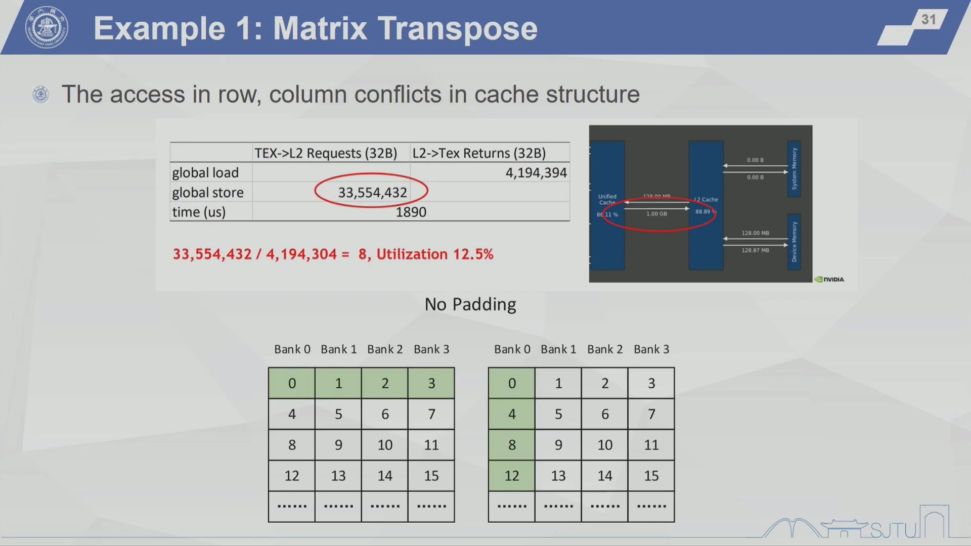
原因不在计算本身,而在访存模式:
- 读 input 时,warp 中相邻 thread 通常读相邻地址,global load 比较连续
- 写 output 时,由于是转置写入,相邻 thread 可能写到相隔很远的地址,global store 变成 stride / scattered access
- 这种行、列访问方向不一致,会在 cache / memory transaction 上产生冲突和低利用率
课件里的指标显示:
也就是说,store 侧请求数量膨胀到理想情况的 8 倍,有效利用率只有 12.5%。这个例子想说明:矩阵转置不是算得慢,而是访存模式拖慢了性能。
优化思路:用 shared memory 做 tile
Programming Model 给我们的优化工具是 thread block 和 shared memory。可以让一个 thread block 负责一个小 tile:
- 先让 thread block 中的 thread 从 global memory 连续读取一个 tile
- 把 tile 放到 shared memory 中
- 在 shared memory 中完成转置
- 再把转置后的 tile 连续写回 global memory
这样做的核心思想是:把“全局内存中的不规则转置访问”拆成“global memory 连续读写 + shared memory 内部重排”。global memory 访问更规整,性能就会好很多。
Dummy padding
但是 shared memory 自己也有 bank。若直接使用 32 x 32 的 shared memory tile,转置访问时可能让多个 thread 落到同一个 bank,形成 bank conflict。
课件给出的解决方式是 dummy padding:
这里不是因为需要真正存 33 列有效数据,而是故意多加一列 padding,使每一行的起始地址错开。这样在按列方向读取 shared memory 时,thread 访问会分散到不同 bank,减少冲突,实现 Bank Parallelism。
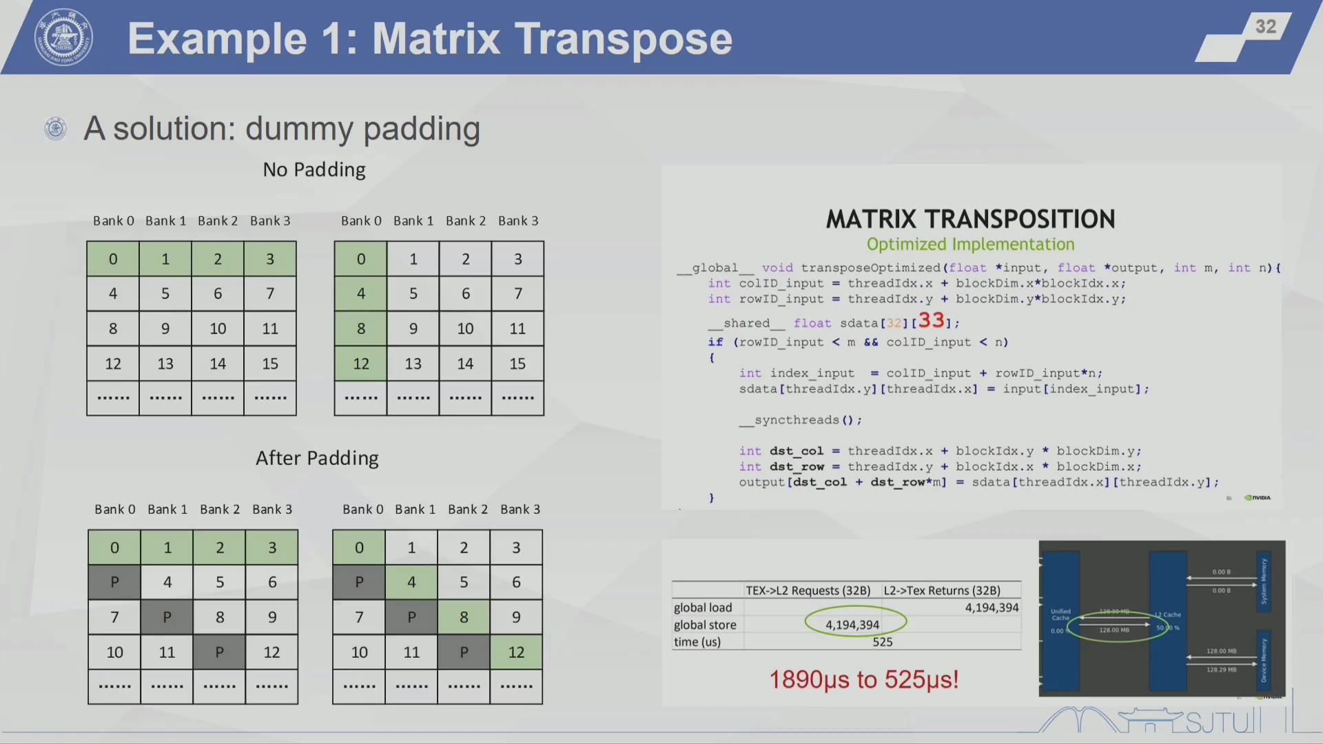
优化后,课件里的 global store 请求从 33,554,432 降到 4,194,394,时间从:
这已经比较接近前面估算的理想访存时间 409.6 us。
4.2 Example 2: Matrix Multiplication
第二个例子是 GEMM(General Matrix Multiplication),也就是矩阵乘法:
其中 K 是 reduction axis。对每个输出元素:
GEMM 在深度学习和 LLM 里非常常见。
这一节不是要深究每一版 kernel 的代码,而是看一个核心问题:怎样根据 GPGPU programming model,把同一个 GEMM 映射到不同层级的硬件资源上,从而逐步提升性能。
从 naive 到 GPU kernel
最朴素的 CPU 版本就是三层循环:
for (int i = 0; i < M; ++i) {
    for (int j = 0; j < N; ++j) {
        float sum = 0.0f;
        for (int k = 0; k < K; ++k) {
            sum += A[i * K + k] * B[k * N + j];
        }
        C[i * N + j] = sum;
    }
}
它直接表达了数学定义,但没有充分利用并行硬件。GPU naive 版本通常让一个 thread 负责一个 C[row, col],thread 内沿 K 方向做 reduction。这样已经能把大量输出元素并行起来,但性能仍然离 A100 的峰值很远,因为每个 thread 都反复从 global memory 读 A 和 B,数据复用没有做好。
Shared memory optimization:减少重复访问 DDR/HBM
矩阵乘法的关键在于复用:
- 同一块
Atile 会被多个C元素使用 - 同一块
Btile 也会被多个C元素使用
如果每个 thread 都直接从 DDR/HBM 读自己需要的数据,就会产生大量重复访问。shared memory 优化的基本思想是:
- 一个 thread block 负责一个
C的 tile - 先把对应的
Atile 和Btile 从 global memory 搬到 shared memory - block 内多个 thread 反复使用 shared memory 中的数据
- 算完当前 tile 后,再进入下一段
Ktile
没有 shared memory 优化时,A 和 B 会从 DDR 中被重复读多次;使用 shared memory 后,global memory 只负责把 tile 搬进来一次,后续复用发生在 shared memory 中。
这对应我们前面学过的 memory model:让高复用数据尽量停留在更靠近计算单元的存储层级里。
Dataflow optimization:让谁 stationary
dataflow optimization 关注的是:在计算 C += A * B 的过程中,应该让哪一类数据尽量停留在片上,减少搬运。
课件列了几种思想:
- Output Stationary:让部分和
C尽量留在寄存器 / 片上,累加完成后再写回 - Input Stationary:让输入
A尽量停留,被多个计算复用 - Weight Stationary:让权重
B尽量停留,被多个计算复用
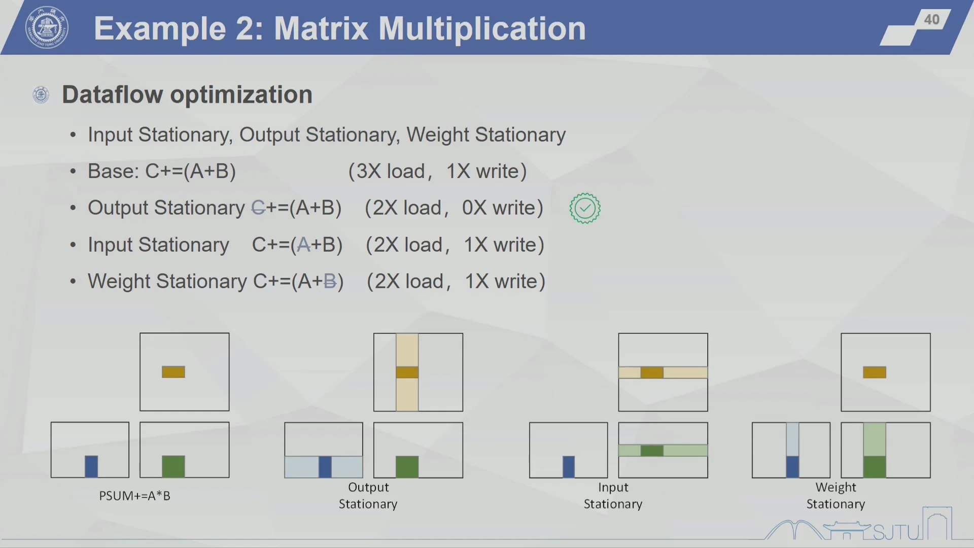
GEMM 中常见且自然的方式是 output stationary:每个 thread / warp 维护一小块 C 的 partial sum,把累加值留在 register file 中,直到 K 方向累加完成后再写回 global memory。这样可以减少对 C 的反复读写。
这个思想和神经网络加速器里常讲的 dataflow 是同一类问题:不是只关心算多少次乘加,还要关心数据在哪一级存储里停留、什么时候移动、被复用多少次。
Tiling:把 GEMM 映射到 memory hierarchy
GEMM 调优的核心形态是多级 tiling:
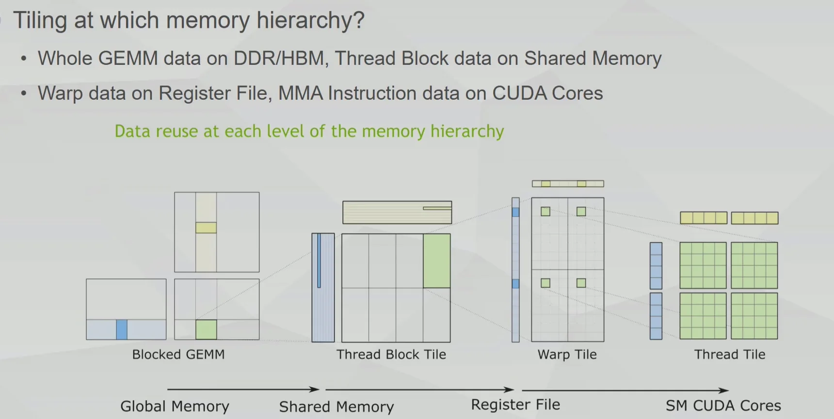
可以按硬件层级来理解:
- 整个 GEMM 数据放在 DDR/HBM,也就是 global memory
- Thread block 负责较大的 tile,并把对应数据搬到 shared memory
- Warp 负责更小的 warp tile,数据进入 register file
- Thread / MMA instruction 负责更小的 thread tile,最终送到 CUDA cores / Tensor Cores 执行
这张图的重点是:每一级 memory hierarchy 都承担一个 tile,每一级都尽量做数据复用。
所以 GEMM 的调优不是简单地“开更多 thread”,而是要设计:
- 一个 block 算多大的
Ctile - 每次搬多大的
A/Btile 到 shared memory - 一个 warp 负责 tile 中的哪一块
- 每个 thread 在 register 中维护多少个 partial sums
- 数据搬运和计算能不能重叠
Tensor Core 和 software pipeline
当使用 Tensor Core 时,单次矩阵乘加的算力会大幅提高。课件中 half-float 的 Tensor Core 版本性能远高于普通 CUDA Core 版本。
但是算得越快,越容易暴露 memory access time:如果数据搬运跟不上,Tensor Core 就会等待数据,产生 stall。因此后面需要 software pipeline 这类技术,让不同阶段重叠:
- 当前 tile 正在计算
- 下一批数据同时从 global memory 搬到 shared memory
- shared memory 中的数据再继续搬到 register
这和前面 memory hierarchy 的思想是一致的:让数据提前到位,让计算单元尽量不断粮。
Performance progression
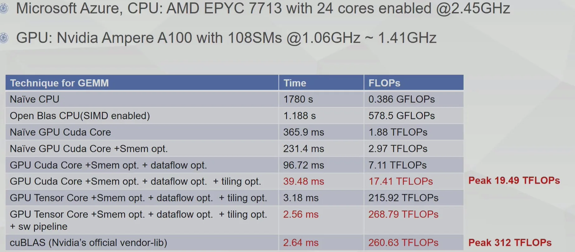
- naive CPU 很慢
- OpenBLAS CPU 通过 SIMD 等优化大幅提升
- naive GPU 已经快很多,但离峰值还有距离
- 加入 shared memory、dataflow、tiling 后,CUDA Core 版本逐步接近 CUDA Core 峰值
- 换用 Tensor Core 后,性能跨到更高量级
- 再加入 software pipeline 后,性能进一步接近 cuBLAS
这个例子的重点可以压缩成一句话:
GEMM 性能调优的本质,是把数据复用按
global memory -> shared memory -> register file -> compute cores逐层安排好,并让计算和搬运尽量重叠。