ViT

0. Abstract¶

尽管Transformer架构已成为自然语言处理任务的事实标准，但其在计算机视觉领域的应用仍存在局限。当前视觉领域中的注意力机制要么与卷积网络结合使用，要么仅替换卷积网络的某些组件而保留其整体架构。我们证明这种对卷积网络的依赖并非必要，直接应用于图像分块序列的纯Transformer模型在图像分类任务中表现优异。当在大规模数据上进行预训练并迁移至多个中型或小型图像识别基准测试（如ImageNet、CIFAR-100、VTAB等）时，视觉Transformer（ViT）相较最先进的卷积网络能取得更优结果，同时所需的训练计算资源显著减少。

I. Introduction¶

基于自注意力机制的架构（尤其是Transformer模型（Vaswani等人，2017））已成为自然语言处理（NLP）领域的首选方案。当前主流方法是在大规模文本语料库上进行预训练，随后针对特定任务的小型数据集进行微调（Devlin等人，2019）。

受自然语言处理领域成功的启发，多项研究尝试将类CNN架构与自注意力机制结合（Wang等，2018；Carion等，2020），部分研究甚至完全取代了卷积操作（Ramachandran等，2019；Wang等，2020a）。虽然这些新模型在理论上具有高效性，但由于采用了特殊的注意力模式，尚未在现代硬件加速器上实现有效扩展。

受到Transformer在自然语言处理领域成功扩展的启发，我们尝试以最少的修改将标准Transformer直接应用于图像处理。具体而言，我们将图像分割为若干图块，并将这些图块的线性嵌入序列作为Transformer的输入。图像块的处理方式与自然语言应用中的tokens完全相同。我们以监督学习的方式训练该模型进行图像分类任务。

当这些模型在中等规模数据集（如ImageNet）上训练且未采用强正则化时，其准确率会略低于同等规模的ResNet模型，差距约为几个百分点。这种看似令人失望的结果或许在意料之中：Transformer模型缺乏卷积神经网络（CNN）固有的部分归纳偏置特性，例如平移等变性和局部性，因此在数据量不足时泛化能力较差。

When trained on mid-sized datasets such as ImageNet without strong regularization, these models yield modest accuracies of a few percentage points below ResNets of comparable size. This seemingly discouraging outcome may be expected: Transformers lack some of the inductive biases inherent to CNNs, such as translation equivariance and locality, and therefore do not generalize well when trained on insufficient amounts of data.

However, the picture changes if the models are trained on larger datasets (14M-300M images). We find that large scale training trumps inductive bias. Our Vision Transformer (ViT) attains excellent results when pre-trained at sufficient scale and transferred to tasks with fewer datapoints. When pre-trained on the public ImageNet-21k dataset or the in-house JFT-300M dataset, ViT approaches or beats state of the art on multiple image recognition benchmarks. In particular, the best model reaches the accuracy of 88:55% on ImageNet, 90:72% on ImageNet-ReaL, 94:55% on CIFAR-100, and 77:63% on the VTAB suite of 19 tasks.

然而，当模型在更大规模的数据集（1400万至3亿张图像）上训练时，情况发生了变化。我们发现大规模训练能够超越归纳偏置的限制。当视觉变换器（ViT）在足够规模的数据上进行预训练，并迁移至数据量较少的任务时，其表现极为出色。在公开的ImageNet-21k数据集或内部JFT-300M数据集上预训练后，ViT在多项图像识别基准测试中接近或超越了现有最佳水平。具体而言，最优模型在ImageNet上达到88.55%的准确率，在ImageNet-ReaL上取得90.72%，在CIFAR-100上达到94.55%，在包含19项任务的VTAB测试套件中获得77.63%的准确率。

II. Related Work¶

Naive application of self-attention to images would require that each pixel attends to every other pixel.
若直接将自注意力机制应用于图像处理，每个像素都需要与其他所有像素建立关联。由于计算成本与像素数量的平方成正比，这种方法难以扩展到实际输入尺寸。

Thus, to apply Transformers in the context of image processing, several approximations have been tried in the past. Parmar et al. (2018) applied the self-attention only in local neighborhoods for each query pixel instead of globally. Such local multi-head dot-product self attention blocks can completely replace convolutions (Hu et al., 2019; Ramachandran et al., 2019; Zhao et al., 2020). In a different line of work, Sparse Transformers (Child et al., 2019) employ scalable approximations to global selfattention in order to be applicable to images. An alternative way to scale attention is to apply it in blocks of varying sizes (Weissenborn et al., 2019), in the extreme case only along individual axes (Ho et al., 2019; Wang et al., 2020a). Many of these specialized attention architectures demonstrate promising results on computer vision tasks, but require complex engineering to be implemented efficiently on hardware accelerators.
为此，研究者尝试了多种近似方案：Parmar等人（2018年）将自注意力限制在每个查询像素的局部邻域内而非全局范围。这类局部多头点积自注意力模块可完全替代卷积操作（Hu等人，2019年；Ramachandran等人，2019年；Zhao等人，2020年）。另一项工作中，稀疏Transformer（Child等人，2019年）采用可扩展的全局自注意力近似方案以适应图像处理需求。另一种扩展注意力的方法是在不同尺寸的区块中应用注意力机制（Weissenborn等人，2019年），极端情况下仅沿单轴方向计算（Ho等人，2019年；Wang等人，2020a年）。虽然这些专用注意力架构在计算机视觉任务中表现优异，但需要复杂的工程实现才能在硬件加速器上高效运行。

Most related to ours is the model of Cordonnier et al. (2020), which extracts patches of size 2 × 2 from the input image and applies full self-attention on top. This model is very similar to ViT, but our work goes further to demonstrate that large scale pre-training makes vanilla transformers competitive with (or even better than) state-of-the-art CNNs. Moreover, Cordonnier et al. (2020) use a small patch size of 2 × 2 pixels, which makes the model applicable only to small-resolution images, while we handle medium-resolution images as well.
与我们工作最相关的是Cordonnier等人（2020年）提出的模型，该模型从输入图像提取2×2尺寸的图块并施加完整自注意力机制。该模型与ViT高度相似，但我们的研究进一步证明：大规模预训练能使标准Transformer模型达到（甚至超越）前沿CNN模型的性能。此外，Cordonnier等人使用的2×2微小图块尺寸仅适用于低分辨率图像，而我们的方法还能处理中等分辨率图像。

There has also been a lot of interest in combining convolutional neural networks (CNNs) with forms of self-attention, e.g. by augmenting feature maps for image classification (Bello et al., 2019) or by further processing the output of a CNN using self-attention, e.g. for object detection (Hu et al., 2018; Carion et al., 2020), video processing (Wang et al., 2018; Sun et al., 2019), image classification (Wu et al., 2020), unsupervised object discovery (Locatello et al., 2020), or unified text-vision tasks (Chen et al., 2020c; Lu et al., 2019; Li et al., 2019).
学界对卷积神经网络（CNN）与自注意力机制的融合也展现出浓厚兴趣，例如通过增强特征图进行图像分类（Bello等人，2019年），或对CNN输出施加自注意力进行目标检测（Hu等人，2018年；Carion等人，2020年）、视频处理（Wang等人，2018年；Sun等人，2019年）、图像分类（Wu等人，2020年）、无监督目标发现（Locatello等人，2020年）以及图文多模态任务（Chen等人，2020c年；Lu等人，2019年；Li等人，2019年）。

我们的研究为超越标准ImageNet规模的大规模图像识别探索增添了新证据。额外数据源的使用有助于在标准基准测试(standard benchmarks)中取得突破性成果（Mahajan等人，2018年；Touvron等人，2019年；Xie等人，2020年）。Sun等人（2017年）研究了CNN性能随数据集规模的变化规律，Kolesnikov等人（2020年）和Djolonga等人（2020年）则对ImageNet-21k和JFT-300M等大型数据集的CNN迁移学习进行了实证探索。我们同样聚焦于这两个数据集，但采用Transformer架构替代了先前工作中基于ResNet的模型。

Transfer Learning¶

把在“旧任务/旧数据”上学到的知识，迁移到“新任务/新数据”上来用。
在深度学习里：

• 旧任务：通常是 大数据集 上训练好的模型（比如 ImageNet、大规模语音/文本数据）
• 新任务：你现在手头的、数据比较少的任务

迁移方式：

• 特征提取（Feature Extraction）
  冻结 backbone（不训练），只训练后面的分类头。
  适合数据很少，新任务和旧任务差别不大的情况
• 微调（Fine-tuning）
  加载预训练模型，然后在新任务上继续训练整个模型（或者部分层）
  适合数据稍多，想获得更高性能的情况

迁移学习的好处：收敛速度快、训练时间大幅减少，不容易出现过拟合，效果往往比从零开始训练好。

可扩展性 Scalability¶

Transformer 架构的一个重要优点是其良好的可扩展性。

什么是scalability可扩展性？
模型的性能上限是否随着资源投入的增加而持续提升
简单来说，一个具有高可扩展性的架构满足以下公式：
更多的数据 + 更大的模型参数量 + 更多的计算算力 = 显著更好的性能
低可扩展性： 当你把模型做大、数据增多时，准确率很快就“饱和”了（不再提升），甚至因为难以训练而下降。
高可扩展性（Transformer）： 只要你敢给它喂更多的数据、把模型层数堆得更高，它的效果就能持续增长，几乎看不到天花板。

为什么 Transformer 架构具有这种可扩展性？
相比于CNN（卷积神经网络）和RNN（循环神经网络），Transformer（以及ViT）具有先天的架构优势：

1. 极高的并行计算效率 (Computational Efficiency)
   对比RNN：RNN必须处理完第1个词才能处理第2个，无法并行。
   对比CNN：虽然CNN可以并行，但深度CNN的感受野扩张需要通过多层堆叠。
   Transformer： 自注意力机制（Self-Attention）的核心是矩阵乘法。它可以一次性并行处理所有的Image Patches。这使得它能完美利用现代GPU/TPU的大规模并行计算能力。在论文中，作者提到ViT训练所需的计算资源实际上比同等性能的ResNet要少（论文Abstract最后一句及Table 2）。
2. 弱归纳偏置 (Less Inductive Bias) —— 这一点最关键
   CNN的限制： CNN被设计成具有“平移不变性”和“局部性”。这是一种人为的“偏见”（Inductive Bias），假设像素只和周围的像素有关。这在数据少时是好事（帮模型省力），但在数据量极度丰富时，这种人为设计的结构反而限制了模型的上限。
   Transformer的自由： ViT几乎没有这种假设。它允许图像中的任意一个Patch直接与另一个Patch建立联系（Global Attention），无论它们相距多远。
   - 代价： 在小数据上难以训练，因为模型需要自己从头学习“什么是空间关系”。
   - 收益： 在大数据上（JFT-300M），因为它不受人为规则的束缚，它能学习到比CNN更复杂、更微妙的全局模式，因此上限更高。

III. Method¶

在模型设计中，我们尽可能严格遵循原始Transformer架构（Vaswani等人，2017）。这种刻意保持简洁的设计有个显著优势：可扩展的NLP Transformer架构及其高效实现几乎可以即插即用。

3.1 Vision Transformer¶

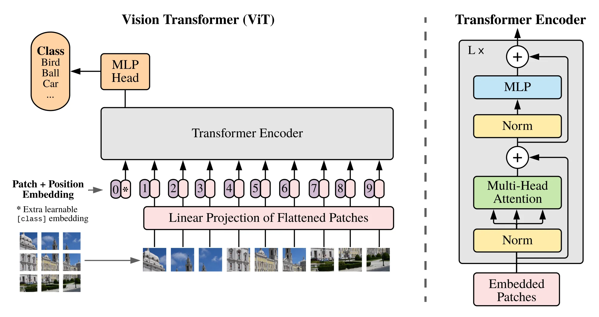
An overview of the model is depicted in Figure 1. The standard Transformer receives as input a 1D sequence of token embeddings. To handle 2D images, we reshape the image \(x \in R^{H\times W \times C}\) into a sequence of flattened 2D patches \(x_p \in R^{N\times(P^2·C)}\), where \((H, W)\) is the resolution of the original image, C is the number of channels, \((P, P)\) is the resolution of each image patch, and \(N = HW/P^2\) is the resulting number of patches, which also serves as the effective input sequence length for the Transformer. The Transformer uses constant latent vector size \(D\) through all of its layers, so we flatten the patches and map to D dimensions with a trainable linear projection (Eq. 1). We refer to the output of this projection as the patch embeddings.
模型概览如图1所示。标准Transformer的输入为一维的token嵌入序列。为处理二维图像，我们将图像\(x \in \mathbb{R}^{H\times W\times C}\)重塑为扁平化的二维图像块序列\(x_p \in \mathbb{R}^{N\times (P^2\cdot C)}\)，其中\((H, W)\)为原始图像分辨率，\(C\)为通道数，\((P, P)\)为每个图像块的分辨率，\(N = HW/P^2\)为处理后图像块的数量，该数值同时作为Transformer的有效输入序列长度。Transformer在所有层中均使用恒定潜向量维度\(D\)，因此我们将图像块展平后通过可训练的线性投影（式1）映射至\(D\)维空间。该投影输出结果称为图像块嵌入。

第一步：从图片到序列（Image to Sequence）¶

——对应论文中的“Patch Embedding”

Transformer最初是用来处理自然语言（文本）的，输入是一串单词（Token）。图片是二维的像素网格，怎么变成一串单词呢？

作者采用了一种简单粗暴的 “切块法”：

1. 切分（Reshape）：

   • 假设你有一张图片 \(\mathbf{x}\)，大小是 \(H \times W \times C\)（例如 \(224 \times 224 \times 3\)）。
   • 设定一个 Patch Size \(P\)（论文标题里的 16x16 就是指 \(P=16\)）。
   • 把图片切成 \(N\) 个固定大小的方块（Patches）。
   • 数量 \(N\)： \(N = HW / P^2\)（例如 \(224^2 / 16^2 = 196\) 个Patch）。
   • 每个Patch的维度： \(P \times P \times C\)（例如 \(16 \times 16 \times 3 = 768\) 个像素值）。

2. 拉平（Flatten）：

   • 把每个Patch里的像素点拉成一条直线，变成一个长向量。
   • 现在的输入变成了 \(N\) 个向量，每个向量长度是 \(P^2 \cdot C\)。

3. 线性映射（Linear Projection of Flattened Patches）：

   • Transformer内部有一个固定的向量维度 \(D\)（Latent vector size，比如 768 或 1024）。
   • 现在的Patch向量长度是像素数（\(P^2 \cdot C\)），通常不等于 \(D\)。
   • 所以，作者用一个可学习的线性层（即公式1中的矩阵 \(\mathbf{E}\)）把每个Patch映射到 \(D\) 维。
   • 结果： 你得到了一串序列，包含 \(N\) 个 \(D\) 维的向量。这在Transformer眼里，和一句话里的 \(N\) 个单词没有任何区别。

第二步：添加身份信息（Class Token & Position Embeddings）¶

——对应公式 (1)

仅仅把图片切碎是不够的，还需要做两个关键操作，才能送入Transformer Encoder。

1. 添加 [class] Token（分类专用标志）：

   • 问题： Transformer输入 \(N\) 个向量，输出也是 \(N\) 个向量。最后到底用哪一个向量来代表整张图片进行分类呢？是取平均吗？
   • 解法： 作者参考了NLP模型 BERT 的做法。在输入序列的最前面，硬塞进去一个可学习的向量（论文中叫 \(\mathbf{x}_{class}\) 或 \(\mathbf{z}_0^0\)）。
   • 作用： 这个向量不对应图片上的任何一块。它的任务是在经过层层Transformer处理时，通过“注意力机制”不断从其他图片Patch那里“收集”有用的信息。
   • 结果： 输入序列长度变成了 \(N+1\)。

2. 添加位置编码（Position Embeddings）：

   • 问题： Transformer 的自注意力机制是没有位置概念的。如果你把图片打乱（比如左上角的Patch换到右下角），Transformer 算出来的结果是一模一样的。这对于图像识别显然不行。
   • 解法： 给每一个Patch向量（包括那个特殊的Class Token）加上一个位置向量（\(\mathbf{E}_{pos}\)）。
   • 细节： 作者使用的是标准的可学习的1D位置编码。尽管图片是2D的，但实验表明直接用1D序列号（1, 2, 3...196）效果就已经很好了，不需要复杂的2D坐标编码（附录D.4有详细讨论）。

因此，我们向 Encoder 传入的 Sequence 为：

其中：

第三步：Encoder 内部¶

ViT 的 Encoder 内部与标准 Transformer 架构基本相同，只有如下细节需要注意：

The Transformer encoder (Vaswani et al., 2017) consists of alternating layers of multiheaded selfattention (MSA, see Appendix A) and MLP blocks (Eq. 2, 3). Layernorm (LN) is applied before every block, and residual connections after every block (Wang et al., 2019; Baevski & Auli, 2019) The MLP contains two layers with a GELU non linearity
Transformer编码器（Vaswani等人，2017）由多头自注意力机制（MSA，见附录A）与多层感知器模块（公式2、3）交替堆叠构成。每个模块前应用层归一化（LN），每个模块后采用残差连接（Wang等人，2019；Baevski & Auli，2019）。该多层感知器包含两个采用GELU非线性激活函数的层级。

运算：
第一段：\(\mathbf{z}_{\ell}^{\prime} =\operatorname{MSA}\left(\operatorname{LN}\left(\mathbf{z}_{\ell-1}\right)\right)+\mathbf{z}_{\ell-1}, \quad \ell=1 \ldots L\)
第二段：\(\mathbf{z}_{\ell} =\operatorname{MLP}\left(\operatorname{LN}\left(\mathbf{z}_{\ell}^{\prime}\right)\right)+\mathbf{z}_{\ell}^{\prime}, \quad \ell=1 \ldots L\)

第四步：架构末端如何完成分类？¶

Similar to BERT’s [class] token, we prepend a learnable embedding to the sequence of embedded patches (\(\mathbf{z}_{0}^0 = \mathbf{x}_{\text{class}}\)), whose state at the output of the Transformer encoder (\(\mathbf{z}_{L}^0\)) serves as the image representation y (Eq. 4). Both during pre-training and fine-tuning, a classification head is attached to \(\mathbf{z}_{L}^0\). The classification head is implemented by a MLP with one hidden layer at pre-training time and by a single linear layer at fine-tuning time.

经过 \(L\) 层 Transformer Encoder 的处理（包含多头自注意力 MSA 和 MLP Block），我们得到了输出序列 \(\mathbf{z}_L\)。

这个输出序列依然包含 \(N+1\) 个向量。

1. 只取第一个向量：

   • 正如前面设计的，我们只关心第0个位置的向量（即对应输入时 [class] token 的那个位置）。
   • 论文公式 (4) 写道：\(\mathbf{y} = \text{LN}(\mathbf{z}_L^0)\)。这里的 \(\mathbf{z}_L^0\) 就是最后一层输出的第一个向量。
   • 原理： 因为在Transformer内部，所有Patch都在和这个Class Token进行交互，模型训练的目标就是让这个 \(\mathbf{z}_L^0\) 浓缩整张图片的分类特征。

2. MLP Head（分类头）：

   • 拿到这个特征向量 \(\mathbf{y}\) 后，接一个多层感知机（MLP）或者线性层。
   • 预训练时（Pre-training）： 接一个带有一个隐藏层的MLP。
   • 微调时（Fine-tuning）： 接一个简单的线性层（Linear Layer），输出维度等于类别数（比如ImageNet是1000）。
   • 最后通过 Softmax 得到分类概率。

Notes¶

Inductive bias. We note that Vision Transformer has much less image specific inductive bias than CNNs. In CNNs, locality, two-dimensional neighborhood structure, and translation equivariance are baked into each layer throughout the whole model. In ViT, only MLP layers are local and translationally equivariant, while the self-attention layers are global. The two-dimensional neighborhood structure is used very sparingly: in the beginning of the model by cutting the image into patches and at fine-tuning time for adjusting the position embeddings for images of different resolution (as described below). Other than that, the position embeddings at initialization time carry no information about the 2D positions of the patches and all spatial relations between the patches have to be learned from scratch.
归纳偏置。我们注意到，视觉变换器（Vision Transformer）相比卷积神经网络（CNN）具有更少的图像特异性归纳偏置。在CNN中，局部性、二维邻域结构和平移等变性被固化在模型的每一层中。而在ViT中，只有多层感知机（MLP）层具备局部性和平移等变性，而自注意力层则是全局性的。二维邻域结构的使用非常有限：仅在模型初始阶段通过将图像切割为patch时，以及在微调阶段为适应不同分辨率图像而调整位置嵌入（如后文所述）时发挥作用。除此之外，初始化阶段的位置嵌入并不包含patch的二维位置信息，所有patch间的空间关系均需从头学习。

Hybrid Architecture. As an alternative to raw image patches, the input sequence can be formed from feature maps of a CNN (LeCun et al., 1989). In this hybrid model, the patch embedding projection \(\mathbf{E}\) (Eq. 1) is applied to patches extracted from a CNN feature map. As a special case, the patches can have spatial size 1x1, which means that the input a sequence is obtained by simply flattening the spatial dimensions of the feature map and projecting to the Transformer dimension. The classification input embedding and position embeddings are added as described above.
混合架构。作为原始图像分块的替代方案，输入序列可由卷积神经网络（CNN，LeCun等人，1989年）的特征图构成。在此混合模型中，分块嵌入投影E（公式1）作用于从CNN特征图提取的分块。特殊情况下，分块空间尺寸可采用1×1，这意味着通过简单展平特征图的空间维度并投影至Transformer维度即可获得输入序列。分类输入嵌入与位置嵌入的添加方式如前所述。

3.2 Fine-Tuning and Higher Resolution¶

Typically, we pre-train ViT on large datasets, and fine-tune to (smaller) downstream tasks. For this, we remove the pre-trained prediction head and attach a zeroinitialized \(D\times K\) feedforward layer, where \(K\) is the number of downstream classes. It is often beneficial to fine-tune at higher resolution than pre-training (Touvron et al., 2019; Kolesnikov et al., 2020). When feeding images of higher resolution, we keep the patch size the same, which results in a larger effective sequence length. The Vision Transformer can handle arbitrary sequence lengths (up to memory constraints), however, the pre-trained position embeddings may no longer be meaningful. We therefore perform 2D interpolation of the pre-trained position embeddings, according to their location in the original image. Note that this resolution adjustment and patch extraction are the only points at which an inductive bias about the 2D structure of the images is manually injected into the Vision Transformer.
通常，我们会在大型数据集上对ViT进行预训练，然后针对（规模较小的）下游任务进行微调。为此，我们会移除预训练的预测头，并附加一个以零初始化的\(D\times K\)前馈层，其中\(K\)代表下游任务的类别数量。相较于预训练阶段，采用更高分辨率进行微调往往能获得更好效果（Touvron等，2019；Kolesnikov等，2020）。当输入更高分辨率的图像时，我们保持图像块尺寸不变，这将导致有效序列长度增加。虽然Vision Transformer能够处理任意长度的序列（受内存限制），但预训练的位置嵌入可能不再具有实际意义。因此，我们会根据这些位置嵌入在原始图像中的坐标，对预训练的位置嵌入进行二维插值处理。需要注意的是，这种分辨率调整和图像块提取操作，是人为将关于图像二维结构的归纳偏置注入Vision Transformer的唯一环节。

IV. Experiments¶

We evaluate the representation learning capabilities of ResNet, Vision Transformer (ViT), and the hybrid. To understand the data requirements of each model, we pre-train on datasets of varying size and evaluate many benchmark tasks. When considering the computational cost of pre-training the model, ViT performs very favourably, attaining state of the art on most recognition benchmarks at a lower pre-training cost. Lastly, we perform a small experiment using self supervision, and show that self-supervised ViT holds promise for the future.
我们评估了ResNet、视觉Transformer（ViT）及其混合架构的表征学习能力。为理解各模型对数据量的需求，我们在不同规模的数据集上进行预训练，并对多项基准任务进行评估。当考虑模型预训练的计算成本时，ViT表现出显著优势——以更低的预训练成本在多数识别基准测试中达到最先进水平。最后，我们通过自监督学习开展小型实验，结果表明自监督ViT在未来具有广阔发展前景。

4.1 Setup¶

Datasets¶

To explore model scalability, we use the ILSVRC-2012 ImageNet dataset with 1k classes and 1.3M images (we refer to it as ImageNet in what follows), its superset ImageNet-21k with 21k classes and 14M images (Deng et al., 2009), and JFT (Sun et al., 2017) with 18k classes and 303M high-resolution images. We de-duplicate the pre-training datasets w.r.t. the test sets of the downstream tasks following Kolesnikov et al. (2020). We transfer the models trained on these dataset to several benchmark tasks: ImageNet on the original validation labels and the cleaned-up ReaL labels (Beyer et al., 2020), CIFAR-10/100 (Krizhevsky, 2009), Oxford IIIT Pets (Parkhi et al., 2012), and Oxford Flowers-102 (Nilsback & Zisserman, 2008). For these datasets, pre-processing follows Kolesnikov et al. (2020).

We also evaluate on the 19-task VTAB classification suite (Zhai et al., 2019b). VTAB evaluates
low-data transfer to diverse tasks, using 1 000 training examples per task. The tasks are divided into
three groups: Natural – tasks like the above, Pets, CIFAR, etc. Specialized – medical and satellite
imagery, and Structured – tasks that require geometric understanding like localization.
数据集。为探究模型的可扩展性，我们采用了以下数据集：包含1000个类别、130万张图像的ILSVRC-2012 ImageNet数据集（下文简称ImageNet）；其超集ImageNet-21k包含2.1万个类别和1400万张图像（Deng等人，2009）；以及包含1.8万个类别、3.03亿张高分辨率图像的JFT数据集（Sun等人，2017）。按照Kolesnikov等人（2020）的方法，我们对预训练数据集进行了去重处理，确保其与下游任务测试集无重叠。我们将基于这些数据集训练的模型迁移至多个基准任务：使用原始验证标签和经过清洗的ReaL标签（Beyer等人，2020）的ImageNet、CIFAR-10/100（Krizhevsky，2009）、Oxford IIIT Pets（Parkhi等人，2012）和Oxford Flowers-102（Nilsback & Zisserman，2008）。针对这些数据集，预处理流程遵循Kolesnikov等人（2020）的方法。我们还评估了19个任务组成的VTAB分类测试集（Zhai等，2019b）。VTAB通过每个任务仅用1000个训练样本的方式，评估模型在多样化任务上的小样本迁移能力。这些任务分为三大类：自然类（如上述Pets、CIFAR等任务）、专业类（医学与卫星图像）以及结构化类（需几何理解能力的任务，如定位）。

Model Variants.¶

Model Variants. We base ViT configurations on those used for BERT (Devlin et al., 2019), as summarized in Table 1. The “Base” and “Large” models are directly adopted from BERT and we add the larger “Huge” model. In what follows we use brief notation to indicate the model size and the input patch size: for instance, ViT-L/16 means the “Large” variant with16×16 input patch size. Note that the Transformer’s sequence length is inversely proportional to the square of the patch size, thus models with smaller patch size are computationally more expensive.
For the baseline CNNs, we use ResNet (He et al., 2016), but replace the Batch Normalization layers (Ioffe & Szegedy, 2015) with Group Normalization (Wu & He, 2018), and used standardized convolutions (Qiao et al., 2019). These modifications improve transfer (Kolesnikov et al., 2020), and we denote the modified model “ResNet (BiT)”. For the hybrids, we feed the intermediate feature maps into ViT with patch size of one “pixel”. To experiment with different sequence lengths, we either (i) take the output of stage 4 of a regular ResNet50 or (ii) remove stage 4, place the same number of layers in stage 3 (keeping the total number of layers), and take the output of this extended stage 3. Option (ii) results in a 4x longer sequence length, and a more expensive ViT model.
模型变体。我们的ViT配置基于BERT（Devlin等人，2019）所使用的架构，如表1所示。其中"Base"和"Large"模型直接沿用BERT的设计，并额外增加了更大规模的"Huge"模型。在下文中，我们采用简写表示模型尺寸与输入图像块大小：例如ViT-L/16代表采用16×16输入图像块的"Large"变体。需注意Transformer的序列长度与图像块尺寸的平方成反比，因此采用较小图像块的模型计算成本更高。
作为基准CNN模型，我们采用ResNet（He等人，2016年），但将批量归一化层（Ioffe & Szegedy，2015年）替换为组归一化（Wu & He，2018年），并使用标准化卷积（Qiao等人，2019年）。这些改进提升了迁移性能（Kolesnikov等人，2020年），我们将改进后的模型记为"ResNet (BiT)"。对于混合架构，我们将中间特征图以单"像素"为图像块尺寸输入ViT。为测试不同序列长度的影响，我们采取两种方案：(i) 直接采用常规ResNet50第4阶段的输出；(ii) 移除第4阶段，在阶段3中放置相同数量的层（保持总层数不变），并采用扩展后阶段3的输出。方案(ii)可使序列长度延长4倍，但会显著增加ViT模型的计算开销。

Training & Fine-tuning¶

We train all models, including ResNets, using Adam (Kingma & Ba, 2015) with \(\beta_1=0.9, \beta_2=0.999\), a batch size of 4096 and apply a high weight decay of 0.1, which we found to be useful for transfer of all models (Appendix D.1 shows that, in contrast to common practices, Adam works slightly better than SGD for ResNets in our setting). We use a linear learning rate warmup and decay, see Appendix B.1 for details. For fine-tuning we use SGD with momentum, batch size 512, for all models, see Appendix B.1.1. For ImageNet results in Table 2, we fine-tuned at higher resolution: 512 for ViT-L/16 and 518 for ViT-H/14, and also used Polyak & Juditsky (1992) averaging with a factor of 0:9999 (Ramachandran et al., 2019; Wang et al., 2020b).
我们采用Adam优化器（Kingma & Ba, 2015）训练所有模型（包括ResNet系列），参数设置为\(\beta_1=0.9, \beta_2=0.999\)，批处理规模为4096，并施加0.1的高权重衰减（附录D.1显示，与常规做法不同，在我们的实验环境下Adam对ResNet的表现略优于SGD）。学习率采用线性预热与衰减策略，详见附录B.1。对于模型微调阶段，所有模型均使用带动量的SGD优化器，批处理规模为512（具体配置参见附录B.1.1）。表2中ImageNet的实验结果采用更高分辨率进行微调：ViT-L/16模型使用512分辨率，ViT-H/14模型使用518分辨率，同时应用Polyak & Juditsky (1992)的滑动平均策略（衰减因子0.9999），该方法参考了Ramachandran等人(2019)和Wang等人(2020b)的工作。

Metrics¶

We report results on downstream datasets either through few-shot or fine-tuning accuracy. Fine-tuning accuracies capture the performance of each model after fine tuning it on the respective dataset. Few-shot accuracies are obtained by solving a regularized least squares regression problem that maps the (frozen) representation of a subset of training images to \(\{-1, 1\}^K\) target vectors. This formulation allows us to recover the exact solution in closed form. Though we mainly focus on fine-tuning performance, we sometimes use linear few-shot accuracies for fast on-the-fly evaluation where fine-tuning would be too costly.
我们在下游数据集上的报告结果采用小样本学习（few-shot）或微调（fine-tuning）准确率两种形式呈现。微调准确率反映了模型在对应数据集上完成微调后的性能表现；小样本学习准确率则通过求解一个正则化最小二乘回归问题获得，该问题将（冻结参数的）训练图像子集表征映射到目标向量\(\{-1, 1\}^K\)。这种数学表达形式使我们能以闭式解获得精确结果。虽然研究主要关注微调性能，但在微调成本过高的场景下，我们偶尔会采用线性小样本学习准确率进行快速实时评估。

4.2 COMPARISON TO STATE OF THE ART¶

我们首先将最大的模型——ViT-H/14和ViT-L/16——与文献中最先进的CNN进行对比。第一个对比对象是Big Transfer（BiT）（Kolesnikov等人，2020年），该研究使用大型ResNet进行监督式迁移学习。第二个对比对象是Noisy Student（Xie等人，2020年），这是一个在去除标签的ImageNet和JFT-300M数据集上通过半监督学习训练的大型EfficientNet。目前，Noisy Student在ImageNet上保持最先进水平，而BiT-L在本文报告的其他数据集上表现最佳。所有模型均在TPUv3硬件上训练，我们报告了每个模型预训练所消耗的TPUv3核心天数（即用于训练的TPU v3核心数——每芯片2个核心——乘以训练天数）。

表2展示了实验结果。在相同JFT-300M数据集上预训练的较小模型ViT-L/16在所有任务中均优于BiT-L，且训练所需计算资源显著减少。更大规模的ViT-H/14模型则进一步提升了性能，尤其在更具挑战性的ImageNet、CIFAR-100和VTAB数据集组上表现突出。值得注意的是，该模型的预训练计算量仍远低于此前最优方法。但需说明，预训练效率不仅受架构选择影响，还与训练计划、优化器、权重衰减等参数相关。我们将在4.4节对不同架构的性能与计算成本进行对照研究。此外，基于公开数据集ImageNet-21k预训练的ViT-L/16模型在多数数据集上也表现优异，其预训练资源消耗更低：使用8核标准云TPUv3约30天即可完成训练。

图2将VTAB任务分解为不同组别，并与该基准测试中的先前最优方法进行对比：包括BiT、基于ImageNet与YouTube联合训练的ResNet变体VIVI（Tschannen等人，2020），以及ImageNet监督与半监督结合的S4L（Zhai等人，2019a）。ViT-H/14在自然场景和结构化任务组中超越了BiT-R152x4及其他方法，而在专业任务组中前两名模型性能相近。

4.3 PRE-TRAINING DATA REQUIREMENTS¶

视觉Transformer（ViT）在大型JFT-300M数据集上预训练时表现优异。相比ResNet，ViT对视觉任务的归纳偏置更少，那么数据集规模究竟有多关键？我们进行了两组实验。

第一组实验中，我们在逐渐增大的数据集（ImageNet、ImageNet-21k和JFT-300M）上预训练ViT模型。为提升小数据集上的性能，我们优化了三个基础正则化参数：权重衰减、dropout和标签平滑。图3展示了微调至ImageNet后的结果（其他数据集结果见表5）。当在最小数据集ImageNet上预训练时，即便采用（适度）正则化，ViT-Large模型表现仍逊于ViT-Base模型；使用ImageNet-21k预训练时两者性能接近；只有在JFT-300M上才能充分体现大模型的优势。图3同时展示了不同规模BiT模型的性能区间：BiT CNN在ImageNet上优于ViT，但随着数据集增大，ViT实现反超。

第二组实验中，我们使用JFT-300M的随机子集（9M、30M、90M）及完整数据集训练模型。小规模子集未额外施加正则化，所有设置采用相同超参数，以此评估模型固有特性而非正则化影响。不过我们采用了早停法，并报告训练过程中的最佳验证准确率。为节省算力，报告的是小样本线性分类准确率而非完整微调结果（图4）。实验表明：在计算成本相近时，视觉Transformer比ResNet更容易在小数据集上过拟合。例如ViT-B/32比ResNet50稍快，在9M子集上表现明显更差，但在90M+子集上更优；ResNet152x2与ViT-L/16也呈现相同规律。这印证了卷积的归纳偏置对小数据集有益，而对大数据集而言，直接从数据中学习相关模式不仅足够，甚至更具优势。

总体而言，ImageNet上的小样本结果（图4）与VTAB上的低数据量结果（表2）显示出ViT在极低数据迁移任务中的潜力。未来工作中对ViT小样本特性的深入分析将是一个值得探索的方向。

4.4 SCALING STUDY¶

我们通过评估从JFT-300M迁移学习的性能，对不同模型进行了受控的规模化研究。在此设定下，数据规模不会成为模型性能的瓶颈，我们重点评估了各模型性能与预训练成本的关系。实验模型组包括：7个ResNet系列（R50x1、R50x2、R101x1、R152x1、R152x2预训练7个周期，以及R152x2和R200x3预训练14个周期）；6个视觉Transformer（ViT-B/32、B/16、L/32、L/16预训练7个周期，加上L/16和H/14预训练14个周期）；以及5个混合模型（R50+ViT-B/32、B/16、L/32、L/16预训练7个周期，外加R50+ViT-L/16预训练14个周期——对于混合模型，名称末尾数字不代表图像分块大小，而是ResNet骨干网络的总下采样率）。

图5展示了迁移性能与总预训练计算量的关系（计算成本细节见附录D.5），附录表6提供了各模型的详细结果。我们观察到几个规律：首先，在性能/计算量权衡方面，视觉Transformer全面优于ResNet。ViT达到相同性能（5个数据集平均值）所需计算量仅为ResNet的1/2至1/4。其次，在较小计算预算时，混合模型略优于ViT，但随着模型规模增大，优势逐渐消失。这一结果有些出人意料，因为通常认为卷积的局部特征处理能力对任何规模的ViT都应有助益。第三，视觉Transformer在实验规模范围内尚未出现性能饱和现象，这为未来的扩展研究提供了动力。

4.5 INSPECTING VISION TRANSFORMER¶

为理解视觉Transformer（ViT）如何处理图像数据，我们首先分析其内部表征机制。ViT的第一层通过线性投影将展平的图像块映射到低维空间（公式1）。图7（左）展示了学习到的嵌入滤波器的主要主成分，这些成分类似于描述每个图像块内部精细结构的低维表示中的合理基函数。

完成投影后，模型会将学习得到的位置编码添加到图像块表征中。图7（中）显示，模型通过位置编码的相似性来编码图像中的空间距离——距离较近的图像块往往具有更相似的位置编码。此外，行列结构特征也得以显现：同一行/列的图像块具有相似的编码。对于更大规模的网格，位置编码还会呈现正弦函数结构（附录D）。这种能自主学习二维图像拓扑的位置编码机制，解释了为何手工设计的二维感知编码变体未能带来性能提升（附录D.4）。

自注意力机制使得ViT即使在最浅层也能整合整幅图像的信息。我们研究了网络对此能力的利用程度：基于注意力权重计算图像空间中信息整合的平均距离（图7右），这种"注意力距离"类似于CNN中的感受野大小。研究发现，部分注意力头在最底层就已关注图像的大部分区域，表明模型确实利用了全局信息整合能力。而另一些注意力头在浅层始终保持较小的注意力距离。这种高度局部化的注意力特征在Transformer前使用ResNet的混合模型中表现较弱（图7右），暗示其功能可能类似于CNN中的早期卷积层。随着网络深度增加，注意力距离逐渐扩大。整体而言，模型关注的图像区域与分类任务语义高度相关（图6）。

4.6 SELF-SUPERVISION¶

Transformer模型在自然语言处理任务中展现出卓越性能。然而，其成功不仅源于出色的可扩展性，更得益于大规模自监督预训练（Devlin等人，2019；Radford等人，2018）。我们同样对掩码补丁预测进行了自监督的初步探索，该方法模拟了BERT中使用的掩码语言建模任务。通过自监督预训练，我们较小的ViT-B/16模型在ImageNet上达到79.9%准确率，相比从头训练显著提升2%，但仍比有监督预训练低4%。附录B.1.2提供了更多细节。我们将对比式预训练（Chen等人，2020b；He等人，2020；Bachman等人，2019；Henaff等人，2020）的研究留待未来工作。

5. Conclusion¶

我们探索了将Transformer架构直接应用于图像识别任务的方法。与先前在计算机视觉领域使用自注意力机制的研究不同，除初始的图像块提取步骤外，我们的架构未引入任何针对图像的特定归纳偏置。取而代之的是，我们将图像视为一系列图像块的序列，并通过自然语言处理中使用的标准Transformer编码器进行处理。当这种简单却可扩展的策略与大规模数据集预训练相结合时，其表现效果出人意料地优异。因此，视觉Transformer模型在多个图像分类数据集上达到或超越了当前最优水平，同时预训练成本相对较低。尽管这些初步成果令人鼓舞，但仍存在诸多挑战：其一是将ViT应用于目标检测和图像分割等其他计算机视觉任务——我们的研究结果与Carion等人（2020）的工作共同印证了该方法的潜力；其二是持续探索自监督预训练方法，虽然初步实验显示自监督预训练已带来性能提升，但其与大规模监督式预训练之间仍存在显著差距；最后，对ViT模型的进一步扩展可能会带来更优的性能表现。